
EP: The contract data used in this analysis was graciously provided by Tom Poraszka, the creator of the now-defunct General Fanager. While the hockey community suffers the loss of yet another tremendous resource, I wish Tom the best of luck with his new venture!
Not a year goes by without at least one NHL contract signing bewildering the hockey world. With healthy scratches making $5MM or more per year, it may seem as though the signing process is just one big roulette spun by managers, players and agents. In reality, though, the NHL player market is remarkably consistent as a whole. We can prove and exploit this fact by leveraging available information to try to predict how much an impending Free Agent will be paid.
Attempts have been made in the past to develop salary prediction models – notably, Matt Cane’s outlined here. Cane uses linear regression to model awarded AAV as a function of various stats belonging to impending Free Agents. As he demonstrates, it is possible to explain a large part of the variance in AAV with this simple regression model.
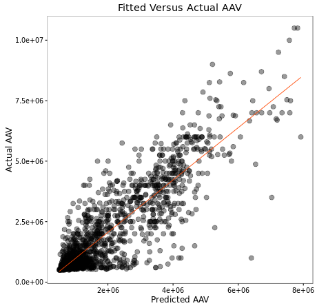
If we look at the predicted vs. actual cap hits for forwards in the graph below, we see that the fit of our model is actually fairly strong, with an R^2 of 0.76, meaning that the 6 variables in our model were able to explain roughly 76% of the variance in UFA cap hits.
It’s worth discussing for a moment the difference between prediction and valuation. Projecting a salary for a pending Free Agent is not the same as appraising them. That is, if a model like Cane’s predicts that a player will earn $3MM, it doesn’t mean the player is worth that much. There is inefficiency in the NHL player market and a good model should capture that.
I decided to look into how we can best guess at how much Free Agents will earn in Average Annual Value. I tested a number of different models and eventually settled on K-Nearest Neighbours.
K-Nearest Neighbours (KNN) is an algorithm that uses the points nearest to a training example to classify or predict a feature of that example. In the 2-dimensional example below, you can view the decision boundary for two values of K:

The classification algorithm works as follows: For each location in space, find the K closest neighbouring points. If the majority of these points belongs to the class red, you would predict a new point in this location to also belong to that class, and vice-versa for class blue. While it is difficult to visualize, this approach extends to any number of dimensions using Euclidean geometry.
Similar to the classification problem, K-Nearest Neighbours can be used to predict features of an arbitrary point in space. This is achieved by taking the average value of that feature for the K closest points. Imagine that each of the points in the diagrams above have a temperature attribute. Now, say we’ve selected two arbitrary locations A and B in the space and identified the 5 nearest points to each. If the temperature values of each of the 5 neighbouring points for both A and B are:
A : [67.1, 68.8, 69.0, 44.7, 59.7]
B : [31.5, 29.4, 44.8, 34.2, 50.1]
then we could predict the temperature attribute for A and B by taking the average:
A : 61.86
B : 38.00
So, what does this mean in hockey terms? Broadly speaking, the idea is to identify the historical Free Agents who most closely resemble a pending Free Agent, and use the average known awarded AAV of those historical cohorts as a prediction for our unknown AAV.
My similarity formula will serve as a method for identifying cohorts. The formula requires weights for each of the statistical parameters, which is where model tuning comes into play. To speed up the process, I perform some manual variable selection beforehand, setting the majority of the weights to zero. Really, all this means is I’ve chosen a small set of stats to compare players by rather than use every metric available to me. The weights and value of K were evaluated by optimizing on the training set using the Nelder-Mead method. In short, the algorithm was responsible for finding the weights to be used in the similarity calculation which minimized the standard error between KNN-predicted AAV and actual AAV. The model’s predictive validity was tested using cross-validation on random folds with a ratio of 80% data for training, 20% for testing.
The complete validation process is outlined below:
- Randomly sample 20% of the Free Agent contract data (the testing set) and keep the remaining 80% (the training set)
- For each of forwards and defensemen, optimize the K value and weights on the training set using the Nelder-Mead algorithm to minimize in-sample error
- Use the optimized weights and K value obtained from the training set to compute the average awarded salary of the K-nearest neighbours to each Free Agent in the testing set
- Compare these averages to the known awarded AAV for each Free Agent in the testing set and log the differences
- Repeat 4 times
- Compute the average error of all trials
The standard error yielded in cross-validation was $638,763, meaning the model predicted the AAV of Free Agents not included in the training data to within $638,763 on average.
Below is a summary of the weights obtained from optimizing over the entire data set:
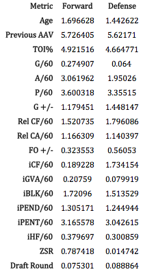
Remember that these weights are not linear coefficients but rather a measure of the importance of that metric in defining similar players. The fact hits are heavily weighted does not mean that players who hit more earn more money. In addition to the weights above, the optimal value for K was found to be 16 in both cases.
While there are several big misses, the vast majority of residuals lie within $1MM of the fitted value:
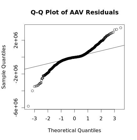
Nearly 85% of the absolute residuals were less than $1MM and nearly 50% were below $250,000. The average in-sample error was roughly $500,000.
The largest discrepancies between fitted and actual AAV values were Dany Heatley’s 2013-14 contract ($5.4M under expected), P.K Subban’s 2013-14 contract ($3.8M above expected), Eric Staal’s 2015-16 contract ($3.5M below expected) and Andrew MacDonald’s 2013-14 contract ($3.3M above expected). The closest fit was Chris Breen’s 2013-14 contract, which earned him just $73 above the fitted value.